


Frozenlake benchmark
In this post we’ll compare a bunch of different map sizes on the FrozenLake environment from the reinforcement learning Gymnasium package using the Q-learning algorithm.
Dependencies
Let’s first import a few dependencies we’ll need.
# Author: Andrea Pierré
# License: MIT License


from pathlib import Path
from typing import NamedTuple

import matplotlib.pyplot as plt
import numpy as np
import pandas as pd
import seaborn as sns
from tqdm import tqdm

import gymnasium as gym
from gymnasium.envs.toy_text.frozen_lake import generate_random_map


sns.set_theme()

# %load_ext lab_black
Parameters we’ll use
class Params(NamedTuple):
    total_episodes: int  # Total episodes
    learning_rate: float  # Learning rate
    gamma: float  # Discounting rate
    epsilon: float  # Exploration probability
    map_size: int  # Number of tiles of one side of the squared environment
    seed: int  # Define a seed so that we get reproducible results
    is_slippery: bool  # If true the player will move in intended direction with probability of 1/3 else will move in either perpendicular direction with equal probability of 1/3 in both directions
    n_runs: int  # Number of runs
    action_size: int  # Number of possible actions
    state_size: int  # Number of possible states
    proba_frozen: float  # Probability that a tile is frozen
    savefig_folder: Path  # Root folder where plots are saved


params = Params(
    total_episodes=2000,
    learning_rate=0.8,
    gamma=0.95,
    epsilon=0.1,
    map_size=5,
    seed=123,
    is_slippery=False,
    n_runs=20,
    action_size=None,
    state_size=None,
    proba_frozen=0.9,
    savefig_folder=Path("../../_static/img/tutorials/"),
)
params

# Set the seed
rng = np.random.default_rng(params.seed)

# Create the figure folder if it doesn't exist
params.savefig_folder.mkdir(parents=True, exist_ok=True)
The FrozenLake environment
env = gym.make(
    "FrozenLake-v1",
    is_slippery=params.is_slippery,
    render_mode="rgb_array",
    desc=generate_random_map(
        size=params.map_size, p=params.proba_frozen, seed=params.seed
    ),
)
Creating the Q-table
In this tutorial we’ll be using Q-learning as our learning algorithm and \(\epsilon\)-greedy to decide which action to pick at each step. You can have a look at the References section for some refreshers on the theory. Now, let’s create our Q-table initialized at zero with the states number as rows and the actions number as columns.
params = params._replace(action_size=env.action_space.n)
params = params._replace(state_size=env.observation_space.n)
print(f"Action size: {params.action_size}")
print(f"State size: {params.state_size}")


class Qlearning:
    def __init__(self, learning_rate, gamma, state_size, action_size):
        self.state_size = state_size
        self.action_size = action_size
        self.learning_rate = learning_rate
        self.gamma = gamma
        self.reset_qtable()

    def update(self, state, action, reward, new_state):
        """Update Q(s,a):= Q(s,a) + lr [R(s,a) + gamma * max Q(s',a') - Q(s,a)]"""
        delta = (
            reward
            + self.gamma * np.max(self.qtable[new_state, :])
            - self.qtable[state, action]
        )
        q_update = self.qtable[state, action] + self.learning_rate * delta
        return q_update

    def reset_qtable(self):
        """Reset the Q-table."""
        self.qtable = np.zeros((self.state_size, self.action_size))


class EpsilonGreedy:
    def __init__(self, epsilon):
        self.epsilon = epsilon

    def choose_action(self, action_space, state, qtable):
        """Choose an action `a` in the current world state (s)."""
        # First we randomize a number
        explor_exploit_tradeoff = rng.uniform(0, 1)

        # Exploration
        if explor_exploit_tradeoff < self.epsilon:
            action = action_space.sample()

        # Exploitation (taking the biggest Q-value for this state)
        else:
            # Break ties randomly
            # Find the indices where the Q-value equals the maximum value
            # Choose a random action from the indices where the Q-value is maximum
            max_ids = np.where(qtable[state, :] == max(qtable[state, :]))[0]
            action = rng.choice(max_ids)
        return action
Running the environment
Let’s instantiate the learner and the explorer.
learner = Qlearning(
    learning_rate=params.learning_rate,
    gamma=params.gamma,
    state_size=params.state_size,
    action_size=params.action_size,
)
explorer = EpsilonGreedy(
    epsilon=params.epsilon,
)
This will be our main function to run our environment until the maximum
number of episodes params.total_episodes. To account for
stochasticity, we will also run our environment a few times.
def run_env():
    rewards = np.zeros((params.total_episodes, params.n_runs))
    steps = np.zeros((params.total_episodes, params.n_runs))
    episodes = np.arange(params.total_episodes)
    qtables = np.zeros((params.n_runs, params.state_size, params.action_size))
    all_states = []
    all_actions = []

    for run in range(params.n_runs):  # Run several times to account for stochasticity
        learner.reset_qtable()  # Reset the Q-table between runs

        for episode in tqdm(
            episodes, desc=f"Run {run}/{params.n_runs} - Episodes", leave=False
        ):
            state = env.reset(seed=params.seed)[0]  # Reset the environment
            step = 0
            done = False
            total_rewards = 0

            while not done:
                action = explorer.choose_action(
                    action_space=env.action_space, state=state, qtable=learner.qtable
                )

                # Log all states and actions
                all_states.append(state)
                all_actions.append(action)

                # Take the action (a) and observe the outcome state(s') and reward (r)
                new_state, reward, terminated, truncated, info = env.step(action)

                done = terminated or truncated

                learner.qtable[state, action] = learner.update(
                    state, action, reward, new_state
                )

                total_rewards += reward
                step += 1

                # Our new state is state
                state = new_state

            # Log all rewards and steps
            rewards[episode, run] = total_rewards
            steps[episode, run] = step
        qtables[run, :, :] = learner.qtable

    return rewards, steps, episodes, qtables, all_states, all_actions
Visualization
To make it easy to plot the results with Seaborn, we’ll save the main results of the simulation in Pandas dataframes.
def postprocess(episodes, params, rewards, steps, map_size):
    """Convert the results of the simulation in dataframes."""
    res = pd.DataFrame(
        data={
            "Episodes": np.tile(episodes, reps=params.n_runs),
            "Rewards": rewards.flatten(order="F"),
            "Steps": steps.flatten(order="F"),
        }
    )
    res["cum_rewards"] = rewards.cumsum(axis=0).flatten(order="F")
    res["map_size"] = np.repeat(f"{map_size}x{map_size}", res.shape[0])

    st = pd.DataFrame(data={"Episodes": episodes, "Steps": steps.mean(axis=1)})
    st["map_size"] = np.repeat(f"{map_size}x{map_size}", st.shape[0])
    return res, st
We want to plot the policy the agent has learned in the end. To do that we will: 1. extract the best Q-values from the Q-table for each state, 2. get the corresponding best action for those Q-values, 3. map each action to an arrow so we can visualize it.
def qtable_directions_map(qtable, map_size):
    """Get the best learned action & map it to arrows."""
    qtable_val_max = qtable.max(axis=1).reshape(map_size, map_size)
    qtable_best_action = np.argmax(qtable, axis=1).reshape(map_size, map_size)
    directions = {0: "←", 1: "↓", 2: "→", 3: "↑"}
    qtable_directions = np.empty(qtable_best_action.flatten().shape, dtype=str)
    eps = np.finfo(float).eps  # Minimum float number on the machine
    for idx, val in enumerate(qtable_best_action.flatten()):
        if qtable_val_max.flatten()[idx] > eps:
            # Assign an arrow only if a minimal Q-value has been learned as best action
            # otherwise since 0 is a direction, it also gets mapped on the tiles where
            # it didn't actually learn anything
            qtable_directions[idx] = directions[val]
    qtable_directions = qtable_directions.reshape(map_size, map_size)
    return qtable_val_max, qtable_directions
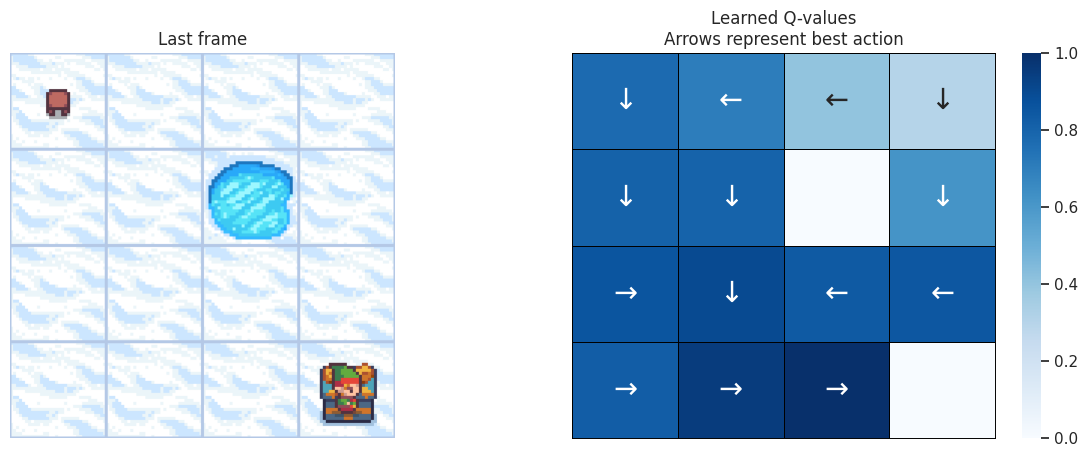
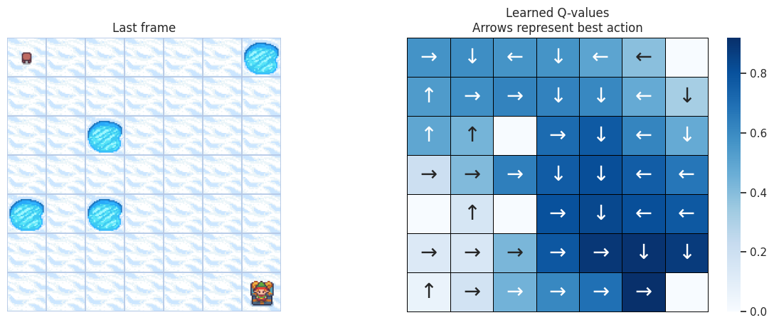
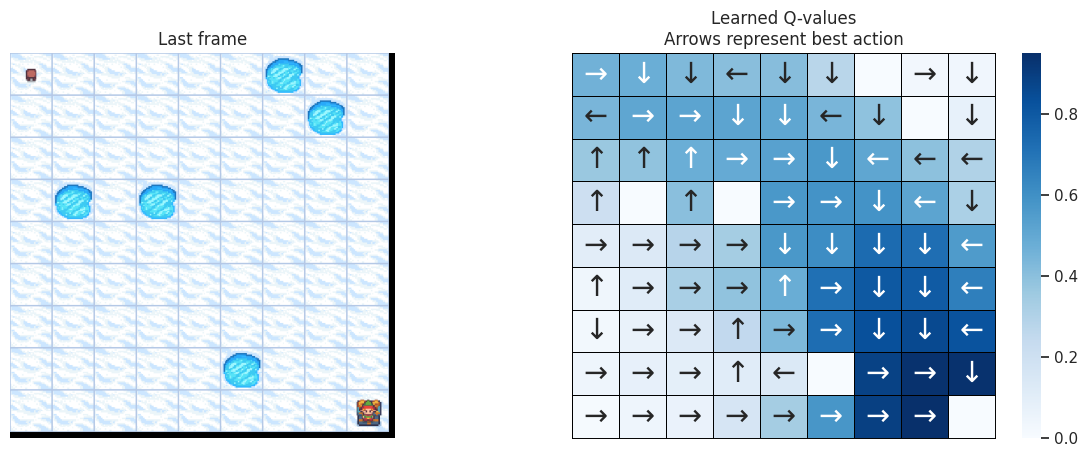
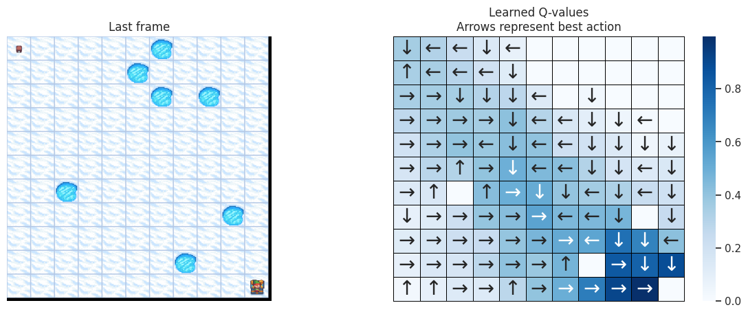
With the following function, we’ll plot on the left the last frame of the simulation. If the agent learned a good policy to solve the task, we expect to see it on the tile of the treasure in the last frame of the video. On the right we’ll plot the policy the agent has learned. Each arrow will represent the best action to choose for each tile/state.
def plot_q_values_map(qtable, env, map_size):
    """Plot the last frame of the simulation and the policy learned."""
    qtable_val_max, qtable_directions = qtable_directions_map(qtable, map_size)

    # Plot the last frame
    fig, ax = plt.subplots(nrows=1, ncols=2, figsize=(15, 5))
    ax[0].imshow(env.render())
    ax[0].axis("off")
    ax[0].set_title("Last frame")

    # Plot the policy
    sns.heatmap(
        qtable_val_max,
        annot=qtable_directions,
        fmt="",
        ax=ax[1],
        cmap=sns.color_palette("Blues", as_cmap=True),
        linewidths=0.7,
        linecolor="black",
        xticklabels=[],
        yticklabels=[],
        annot_kws={"fontsize": "xx-large"},
    ).set(title="Learned Q-values\nArrows represent best action")
    for _, spine in ax[1].spines.items():
        spine.set_visible(True)
        spine.set_linewidth(0.7)
        spine.set_color("black")
    img_title = f"frozenlake_q_values_{map_size}x{map_size}.png"
    fig.savefig(params.savefig_folder / img_title, bbox_inches="tight")
    plt.show()
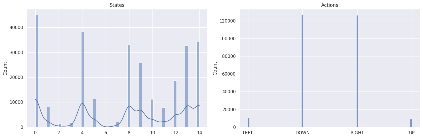
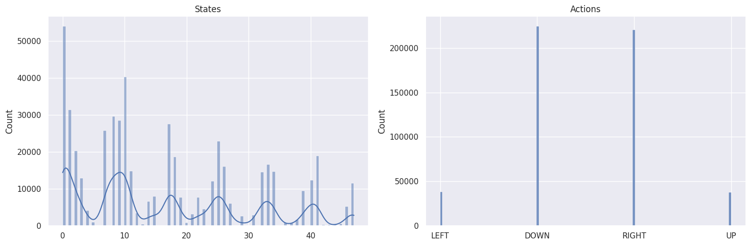
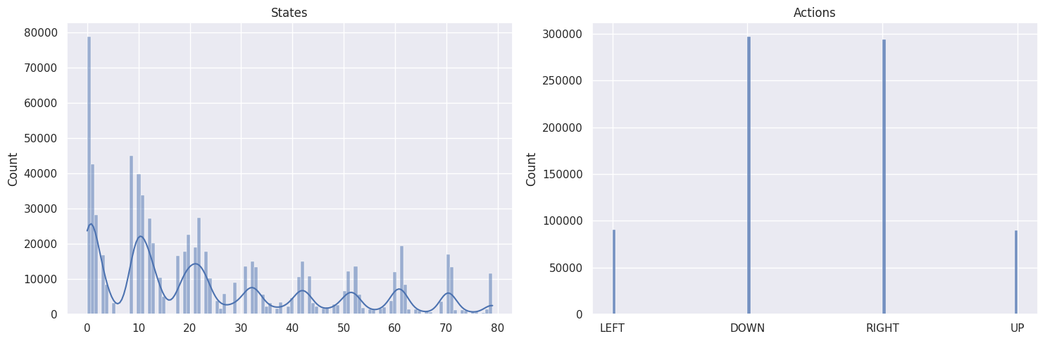
As a sanity check, we will plot the distributions of states and actions with the following function:
def plot_states_actions_distribution(states, actions, map_size):
    """Plot the distributions of states and actions."""
    labels = {"LEFT": 0, "DOWN": 1, "RIGHT": 2, "UP": 3}

    fig, ax = plt.subplots(nrows=1, ncols=2, figsize=(15, 5))
    sns.histplot(data=states, ax=ax[0], kde=True)
    ax[0].set_title("States")
    sns.histplot(data=actions, ax=ax[1])
    ax[1].set_xticks(list(labels.values()), labels=labels.keys())
    ax[1].set_title("Actions")
    fig.tight_layout()
    img_title = f"frozenlake_states_actions_distrib_{map_size}x{map_size}.png"
    fig.savefig(params.savefig_folder / img_title, bbox_inches="tight")
    plt.show()
Now we’ll be running our agent on a few increasing maps sizes: - \(4 \times 4\), - \(7 \times 7\), - \(9 \times 9\), - \(11 \times 11\).
Putting it all together:
map_sizes = [4, 7, 9, 11]
res_all = pd.DataFrame()
st_all = pd.DataFrame()

for map_size in map_sizes:
    env = gym.make(
        "FrozenLake-v1",
        is_slippery=params.is_slippery,
        render_mode="rgb_array",
        desc=generate_random_map(
            size=map_size, p=params.proba_frozen, seed=params.seed
        ),
    )

    params = params._replace(action_size=env.action_space.n)
    params = params._replace(state_size=env.observation_space.n)
    env.action_space.seed(
        params.seed
    )  # Set the seed to get reproducible results when sampling the action space
    learner = Qlearning(
        learning_rate=params.learning_rate,
        gamma=params.gamma,
        state_size=params.state_size,
        action_size=params.action_size,
    )
    explorer = EpsilonGreedy(
        epsilon=params.epsilon,
    )

    print(f"Map size: {map_size}x{map_size}")
    rewards, steps, episodes, qtables, all_states, all_actions = run_env()

    # Save the results in dataframes
    res, st = postprocess(episodes, params, rewards, steps, map_size)
    res_all = pd.concat([res_all, res])
    st_all = pd.concat([st_all, st])
    qtable = qtables.mean(axis=0)  # Average the Q-table between runs

    plot_states_actions_distribution(
        states=all_states, actions=all_actions, map_size=map_size
    )  # Sanity check
    plot_q_values_map(qtable, env, map_size)

    env.close()
Map size: \(4 \times 4\)
Map size: \(7 \times 7\)
Map size: \(9 \times 9\)
Map size: \(11 \times 11\)
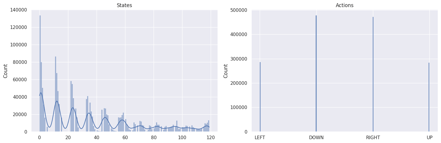
The DOWN and RIGHT actions get chosen more often, which makes
sense as the agent starts at the top left of the map and needs to find
its way down to the bottom right. Also the bigger the map, the less
states/tiles further away from the starting state get visited.
To check if our agent is learning, we want to plot the cumulated sum of rewards, as well as the number of steps needed until the end of the episode. If our agent is learning, we expect to see the cumulated sum of rewards to increase and the number of steps to solve the task to decrease.
def plot_steps_and_rewards(rewards_df, steps_df):
    """Plot the steps and rewards from dataframes."""
    fig, ax = plt.subplots(nrows=1, ncols=2, figsize=(15, 5))
    sns.lineplot(
        data=rewards_df, x="Episodes", y="cum_rewards", hue="map_size", ax=ax[0]
    )
    ax[0].set(ylabel="Cumulated rewards")

    sns.lineplot(data=steps_df, x="Episodes", y="Steps", hue="map_size", ax=ax[1])
    ax[1].set(ylabel="Averaged steps number")

    for axi in ax:
        axi.legend(title="map size")
    fig.tight_layout()
    img_title = "frozenlake_steps_and_rewards.png"
    fig.savefig(params.savefig_folder / img_title, bbox_inches="tight")
    plt.show()


plot_steps_and_rewards(res_all, st_all)
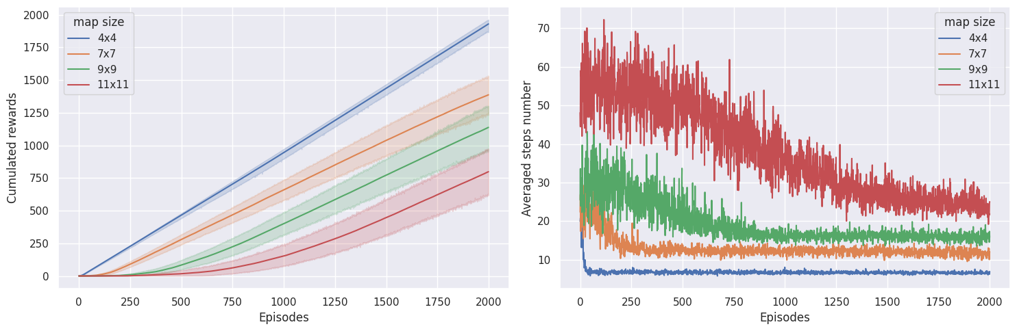
On the \(4 \times 4\) map, learning converges pretty quickly, whereas on the \(7 \times 7\) map, the agent needs \(\sim 300\) episodes, on the \(9 \times 9\) map it needs \(\sim 800\) episodes, and the \(11 \times 11\) map, it needs \(\sim 1800\) episodes to converge. Interestingly, the agent seems to be getting more rewards on the \(9 \times 9\) map than on the \(7 \times 7\) map, which could mean it didn’t reach an optimal policy on the \(7 \times 7\) map.
In the end, if agent doesn’t get any rewards, rewards don’t get
propagated in the Q-values, and the agent doesn’t learn anything. In my
experience on this environment using \(\epsilon\)-greedy and those
hyperparameters and environment settings, maps having more than
\(11 \times 11\) tiles start to be difficult to solve. Maybe using a
different exploration algorithm could overcome this. The other parameter
having a big impact is the proba_frozen, the probability of the tile
being frozen. With too many holes, i.e. \(p<0.9\), Q-learning is
having a hard time in not falling into holes and getting a reward
signal.
References
Code inspired by Deep Reinforcement Learning Course by Thomas Simonini (http://simoninithomas.com/)
David Silver’s course in particular lesson 4 and lesson 5
Q-Learning: Off-Policy TD Control in Reinforcement Learning: An Introduction, by Richard S. Sutton and Andrew G. Barto
Introduction to Reinforcement Learning by Tim Miller (University of Melbourne)